Engineering TTS Inference in vLLM-Omni
vLLM-Omni started with support for omni-modality models and has since expanded to several text-to-speech systems, including Qwen3-TTS, VoxCPM2, Fish Speech S2 Pro, and Higgs Audio V3. This post describes the concrete engineering problems we ran into while adapting and optimizing these models, the solutions we used, and the engineering tradeoffs behind them.
How TTS Inference Differs from Traditional LLM Inference
TTS and text-only LLM inference both use autoregressive models, but the serving bottlenecks are different.
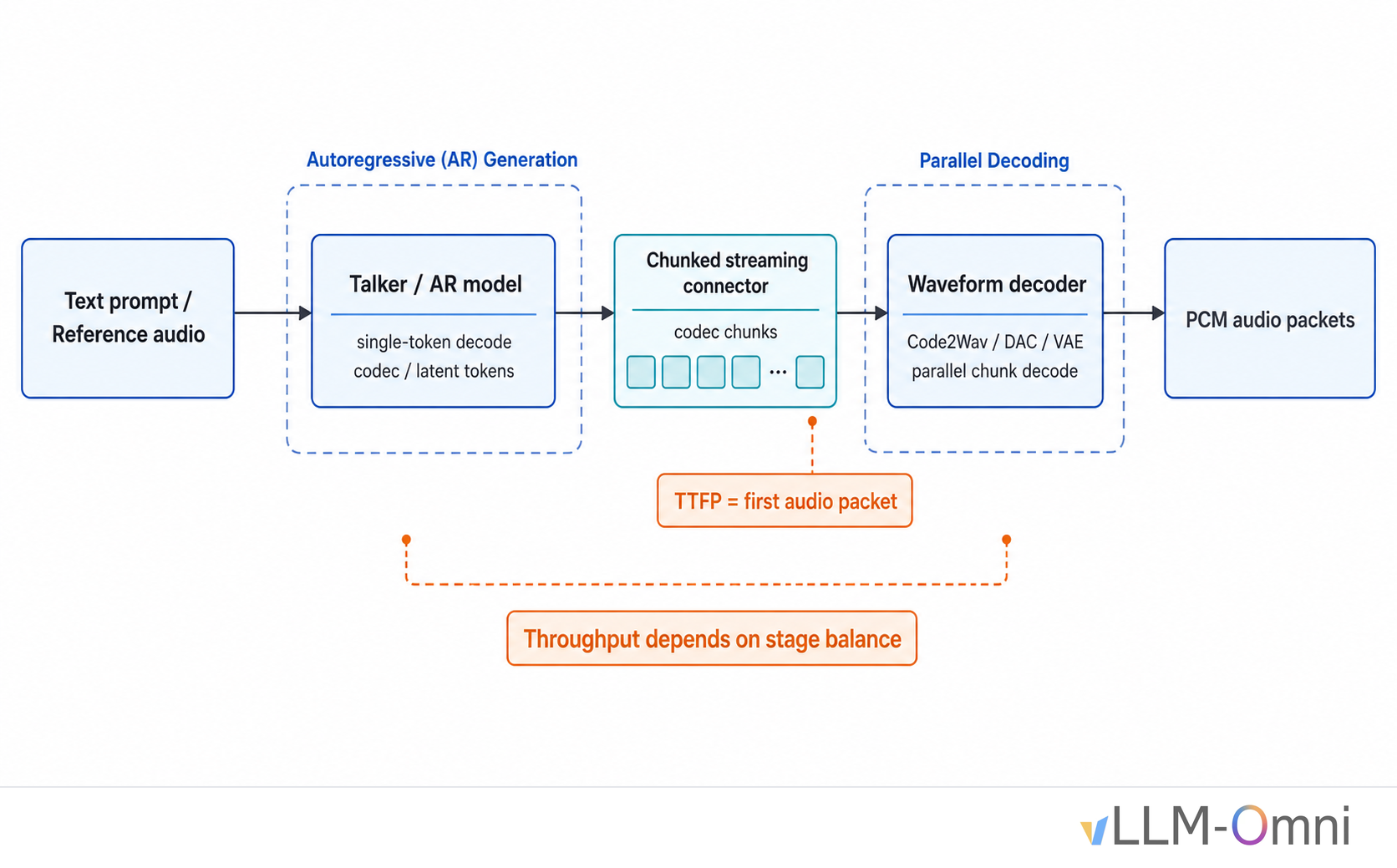
TTS is a pipeline, usually with multiple model stages. A typical TTS system has at least two stages: a Talker predicts codec tokens autoregressively, and a Code2Wav module reconstructs waveform audio from those codec tokens. These stages have very different compute profiles. The Talker is a latency-bound single-token decode workload, while Code2Wav is a throughput-bound parallel decoder. If the scheduler treats the two stages the same way, Talker latency blocks Code2Wav input, and Code2Wav parallelism remains underused. Both latency and throughput suffer.
Streaming output has a strict latency budget. In speech synthesis, users expect to hear the first audio packet within a few hundred milliseconds. The connector layer must support chunked streaming, and chunk size directly affects TTFP, or Time To First Audio Packet. If chunks are too small, Code2Wav does not have enough context to keep audio continuous across chunk boundaries. If chunks are too large, first-packet latency becomes unacceptable.
Throughput still matters. In online serving, how much concurrency a single GPU can sustain, and how many seconds of audio it can generate per wall-clock second, directly determines deployment cost. TTS throughput optimization is more complex than LLM throughput optimization because Talker and Code2Wav have different bottlenecks, and the connector between them adds its own transfer cost. Improving throughput means balancing the two stages while removing the bottlenecks inside each one.
Optimization Overview
Different TTS models have different bottlenecks. vLLM-Omni does not apply one fixed optimization recipe to every model. Instead, we choose optimizations based on each model's pipeline structure, decode state, batch shapes, and numerical constraints.
| Technique | Applies to | Why it matters |
|---|---|---|
| Stage separation and connector chunking | Qwen3-TTS, Higgs Audio V3 | Lets Talker latency and Code2Wav throughput be tuned independently. |
| Batched decode preprocessing | Qwen3-TTS | Reduces repeated per-request Python work in the Talker decode hot path. |
Whole-forward torch.compile | VoxCPM2 | Lets Dynamo see more of the MiniCPM4 forward loop and reduces Python-to-compiled boundaries. |
| CFM/LocDiT decode-tail batching | VoxCPM2 | Turns many tiny per-request diffusion calls into larger GPU batches. |
| GPU-resident decode state | Higgs Audio V3 | Moves multi-codebook state updates out of Python loops and reduces synchronization. |
| Model-specific q_len=1 attention | Fish Speech S2 Pro | Specializes pure decode attention instead of paying for generic paged/varlen paths. |
The important point is that not every optimization works for every TTS architecture. The engineering challenge is choosing the right lever for the right model shape.
Qwen3-TTS: A Full Optimization Path
Qwen3-TTS is a speech generation model family from the Qwen team. It uses a discrete multi-codebook language-model architecture and a 12 Hz tokenizer for acoustic compression and high-fidelity reconstruction1. Its three variants—Base for voice cloning, CustomVoice for predefined speakers with instruction-based emotion and style control, and VoiceDesign for designing new voices from natural-language descriptions of timbre, emotion, and prosody—share the same two-stage architecture: Talker predicts codec tokens autoregressively, and Code2Wav decodes them in parallel. Qwen3-TTS Code2Wav is a lightweight non-DiT decoder and does not require the iterative denoising loop used by diffusion models.
Among the four models discussed here, Qwen3-TTS has the most standard pipeline shape: Talker → connector → Code2Wav. That makes it a useful example for walking through the full TTS inference optimization process.
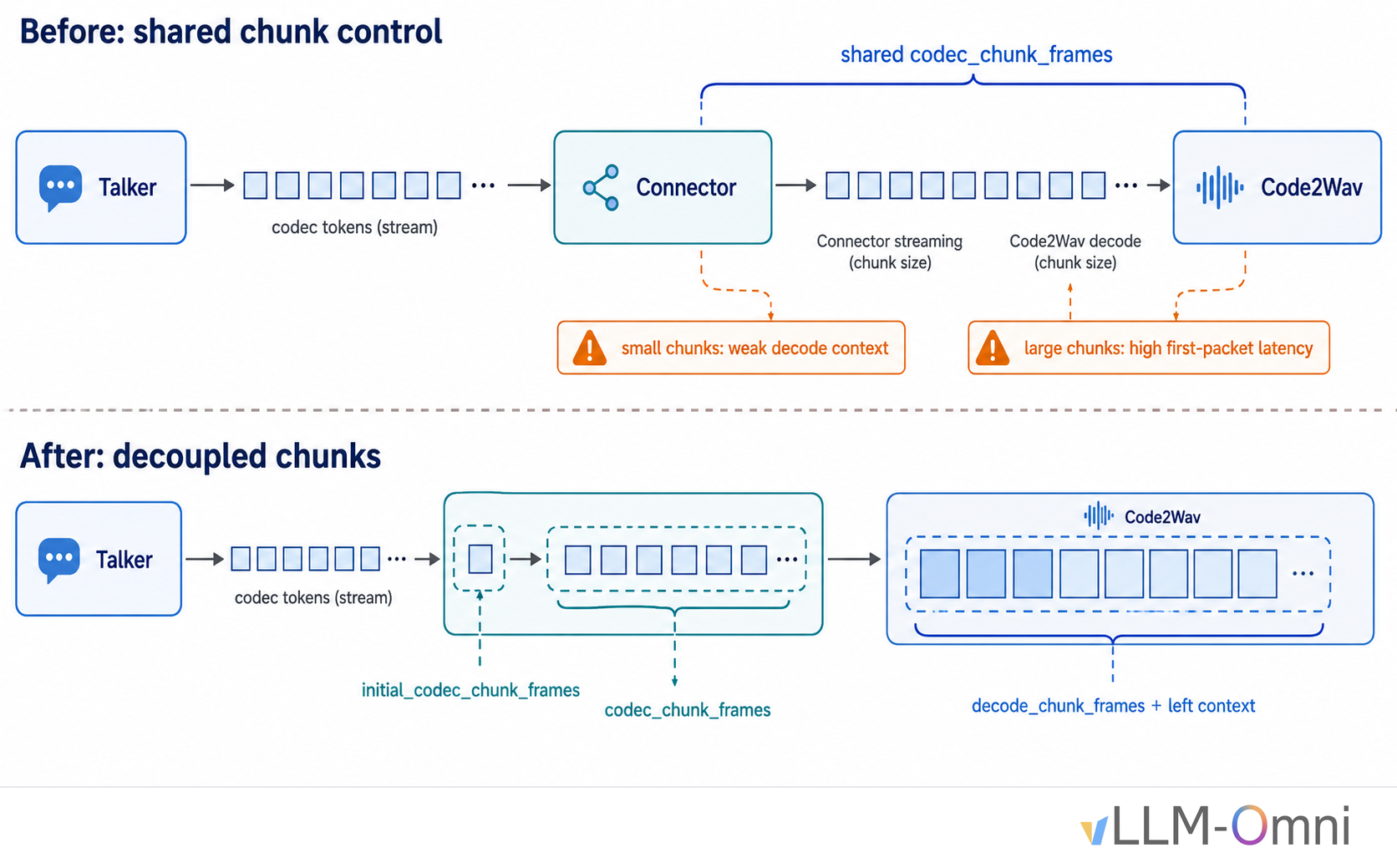
1. Streaming: Decoupling Connector Chunks from the Code2Wav Decode Window
The first optimization target was streaming output. In the early Qwen3-TTS implementation, connector streaming chunks and Code2Wav decode chunks were tied to the same chunk parameter, mainly codec_chunk_frames.
The connector sends codec tokens from Talker to Code2Wav. In streaming mode, if the connector sends very small chunks, Code2Wav also sees very small decode chunks, which hurts cross-chunk audio continuity. If we increase the chunk size for audio quality, first-packet latency increases.
We decoupled the two responsibilities by introducing separate parameters:
codec_chunk_frames: connector streaming chunk size, controlling the Talker-to-Code2Wav transfer cadence.decode_chunk_framesanddecode_left_context_frames: Code2Wav internal decode window and left context, kept independent from connector chunking.initial_codec_chunk_frames: a smaller first codec chunk so Code2Wav can start earlier, after which later chunks return to the regular size.
With this design, the connector can use a small chunk size to reduce first-packet latency, while Code2Wav keeps a 300-frame decode window plus 25 frames of left context to preserve cross-chunk quality. The two knobs can be tuned independently2.
2. Throughput: Stage 0 Decode Preprocessing
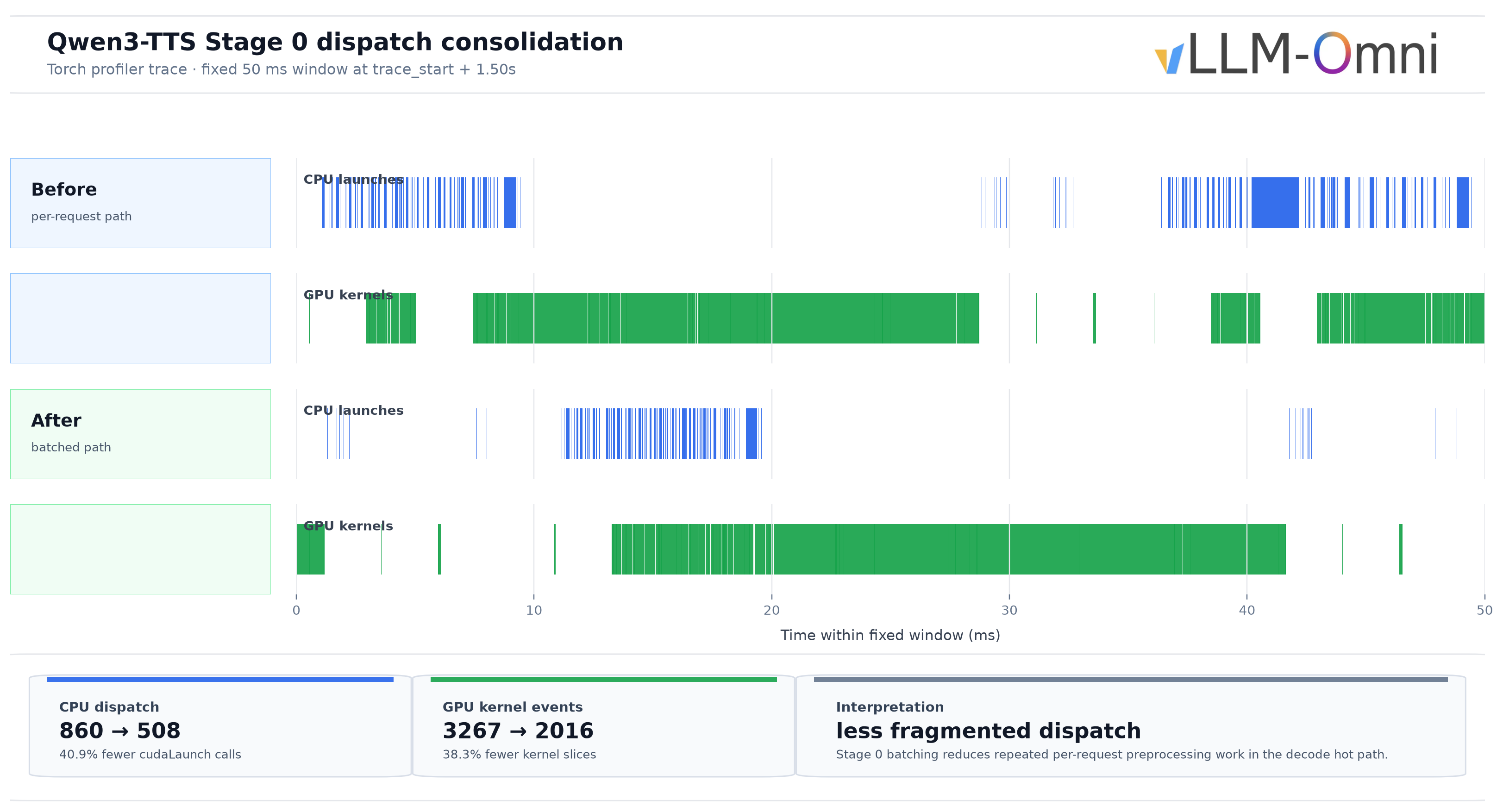
After fixing streaming latency, the next bottleneck was throughput. The first obstacle was the Talker decode loop. Each Qwen3-TTS Talker decode step needs request-level preprocessing: speaker embedding preparation, trailing_text maintenance, and input embedding construction. At c=1 this overhead is small. At c=64, every decode step loops over 64 requests, and Python-side loops plus tensor slicing become visible bottlenecks.
To locate the cost, we profiled Talker decode on H20 × 2 with voice cloning at c=64. In a warm run before the broader hot-path optimizations, the model-external Python and runner-side work—including preprocess_decode_batch, make_omni_output, process_additional_info, build_mm_cpu, and bookkeeping sync—was in the millisecond range per decode step. A few milliseconds per step does not look large in isolation, but one utterance can require roughly 200 decode steps. At c=64, that cost repeats throughout the whole sequence and becomes a significant part of end-to-end latency.
GPU utilization tells the same story. With nvidia-smi sampled at c=64, the baseline average GPU utilization for Stage 0 and Stage 1 was about 14% and 6%, respectively. The GPU was often waiting on Python scheduling, small tensor allocation, and kernel launch overhead rather than compute. This is why the bottleneck was not raw GPU FLOPs but serving-path overhead.
The first concrete target was speaker embedding preparation. In Qwen3-TTS voice-clone mode, each request uses reference audio to extract a speaker embedding and then performs mel/STFT work during decode. The original path computed mel spectrograms per request on CPU and copied them to GPU. At high concurrency, this became many small CPU-to-GPU transfers and kernel launches. We cached the mel basis and window buffers on GPU and batched the mel/STFT computation on GPU, removing repeated CPU work and H2D transfers.
The next target was trailing_text. During decode, the Talker maintains a trailing_text sliding window that caches embeddings for generated tokens. Each decode step appends the current token embedding and removes the oldest token. The original implementation used tensor slicing and concatenation, allocating a new tensor frequently. The optimized path tracks an offset and only compacts when the offset crosses a threshold or reaches the end of the buffer (_TRAILING_TEXT_COMPACT_MIN_FRAMES = 64). Intermediate decode steps index by offset without allocating a new tensor.
The batched preprocess_decode_batch path removed one major source of per-request decode overhead3. The final throughput numbers below come from the stacked optimization path, including Stage 0 batching, connector changes, async D2H, runner hot-path cleanup, and CUDA Graph tuning423. In the final stacked run, Qwen3-TTS audio throughput on H20 × 2 improved from 26.55 audio-s/s to 42.88 audio-s/s (+61.5%), while P99 E2EL dropped from 17.7s to 9.0s.
3. Hot-Path Cleanup
After preprocessing was batched, the remaining profile showed many small Python overheads. Each one is small, but they add up in a high-frequency c=64 decode loop.
req_id_to_index previously used req_ids.index(), turning lookups into an O(N²) list scan inside every decode step. Replacing it with a dictionary made lookup O(1). Non-streaming requests do not need to walk the per-output streaming path in the orchestrator, so we skip that path early. The codec-disallowed mask is precomputed into a buffer, allowing compute_logits to use masked_fill directly instead of rebuilding the mask each time4.
Qwen3-TTS uses CUDA Graph in several places. The Talker code predictor has its own graph path depending on the deploy profile. Here we focus on the Code2Wav decoder CUDA Graph. The decoder input shape is (batch, num_quantizers, codec_frames). In chunked decode, codec_frames has a small set of values: streaming chunk plus left context, non-streaming decode_chunk_frames + decode_left_context_frames (300 + 25 = 325), and tail chunks. These values can be enumerated during warmup. CUDAGraphDecoderWrapper captures graphs by (batch_size, frames) and uses bisect_left at inference time to select the nearest padded bucket. If no graph matches, it falls back to eager execution.
In repeated c=16 tests with qwen3_tts.yaml, Code2Wav CUDA Graph hit rate started at 88% and settled around 81% after five consecutive rounds. The main single-sample shapes, such as (1, 98) -> 169, (1, 73) -> 73, (1, 123) -> 169, and (1, 325) -> 325, hit the captured buckets. Fallbacks mostly came from batch-size > 1 shapes such as (2, 98, 169) and (8, 73, 73). Across the run, stream_capture_fallbacks=0, so no fallback was caused by stream capture failure.
4. Numerical Precision: fp32 Alignment for the Code Predictor
The Talker code predictor has a precision-sensitive path. It works on very short sequences, typically 2–8 tokens, and repeatedly performs prefill. vLLM fused kernels in bfloat16 can differ slightly from the reference implementation. In this short-sequence, high-frequency path, those small differences accumulate and can affect audio quality after dozens of steps.
The fix was to split the code predictor layers and keep selected operations in fp32: RMSNorm variance, RoPE cos/sin, attention, and QKV projection use PyTorch-native implementations for bit-level alignment with the reference path.
5. Validation
After stacking these optimizations, Qwen3-TTS on H20 × 2 at c=64 for voice cloning improved audio throughput by 61.5%, while P99 end-to-end latency dropped by nearly half. The full numbers are in the performance section.
We also ran a warm concurrency sweep with H20 × 2, voice cloning, and streaming output:
| c | Mean TTFP | Mean E2E | P50 TTFP | P50 E2E |
|---|---|---|---|---|
| 1 | 70.61ms | 564ms | 70.61ms | 564ms |
| 8 | 268.75ms | 1.55s | 287.15ms | 1.70s |
| 16 | 451.32ms | 2.62s | 516.15ms | 2.75s |
| 32 | 637.43ms | 5.05s | 634.22ms | 5.10s |
| 64 | 1127.93ms | 8.73s | 1051.05ms | 8.78s |
From c=1 to c=64, E2E grows from 0.56s to 8.73s, not linearly by 64×. Warm high-concurrency serving amortizes fixed costs, but at c=64, Talker and scheduling paths still become a major source of queueing. This is why hot-path cleanup and CUDA Graph remain important.
VoxCPM2: Single-Stage Hybrid TTS
VoxCPM2 is a tokenizer-free TTS model from OpenBMB. It uses a diffusion-autoregressive hybrid design and runs in the latent space of AudioVAE V25. Its Talker is a four-part cascade:
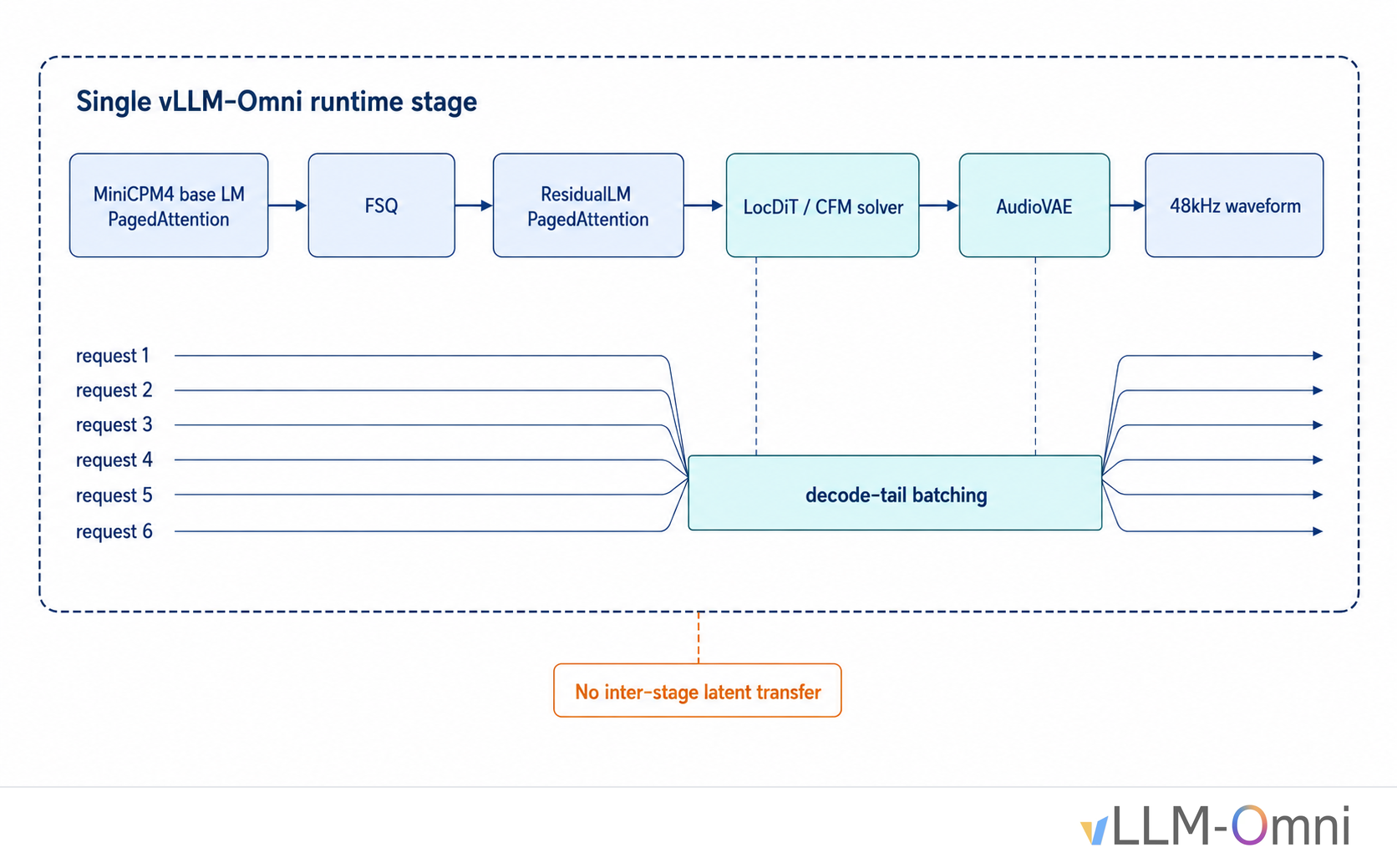
MiniCPM4 (28 layers, PagedAttention) → FSQ → MiniCPM4 ResidualLM (8 layers) → LocDiT (CFM solver) → AudioVAELocDiT performs CFM, or Conditional Flow Matching, diffusion denoising, and AudioVAE reconstructs 48 kHz waveform audio. In vLLM-Omni, VoxCPM2 is not split into multiple runtime stages. Instead, it runs as a single-stage AR TTS pipeline: MiniCPM4, FSQ, ResidualLM, LocDiT, and AudioVAE all execute inside one model instance, and the model directly emits audio. This avoids latent transfer between stages and makes cross-request batching easier for the decode-tail CFM/LocDiT and VAE paths.
Exploring torch.compile
The 28-layer MiniCPM4 is the heaviest part of the VoxCPM2 Talker, so the first optimization target was torch.compile. The path that worked best was not the one we expected initially.
The first attempt compiled each layer's mlp and o_proj separately: 28 layers × 2 modules = 56 compiled regions with fullgraph=True6. The problem is that Dynamo cannot optimize across compiled-region boundaries. Each boundary adds a Python → compiled → Python transition, and 56 regions mean many transitions per decode step.
We then wrapped the entire Model.forward in torch.compile with fullgraph=False7. This lets Dynamo see the full 28-layer loop. PagedAttention still causes graph breaks, but Dynamo only needs to memoize a small number of subgraphs. Per-step dispatch drops from many small regions to a few larger regions. RTF dropped from roughly 0.21 to roughly 0.13, making this the largest single optimization for VoxCPM2.
To quantify this, we profiled three configurations: eager, per-layer compile, and whole/unified graph. Per-layer compile reduced part of the kernel count and kernel time, but launch count did not drop. Whole/unified graph was the key step: cudaLaunchKernel count dropped by about 71%, kernel events by about 30%, and kernel time by about 27%. Single-request E2E dropped by about 2.6% for per-layer compile and about 6.5% for whole graph.
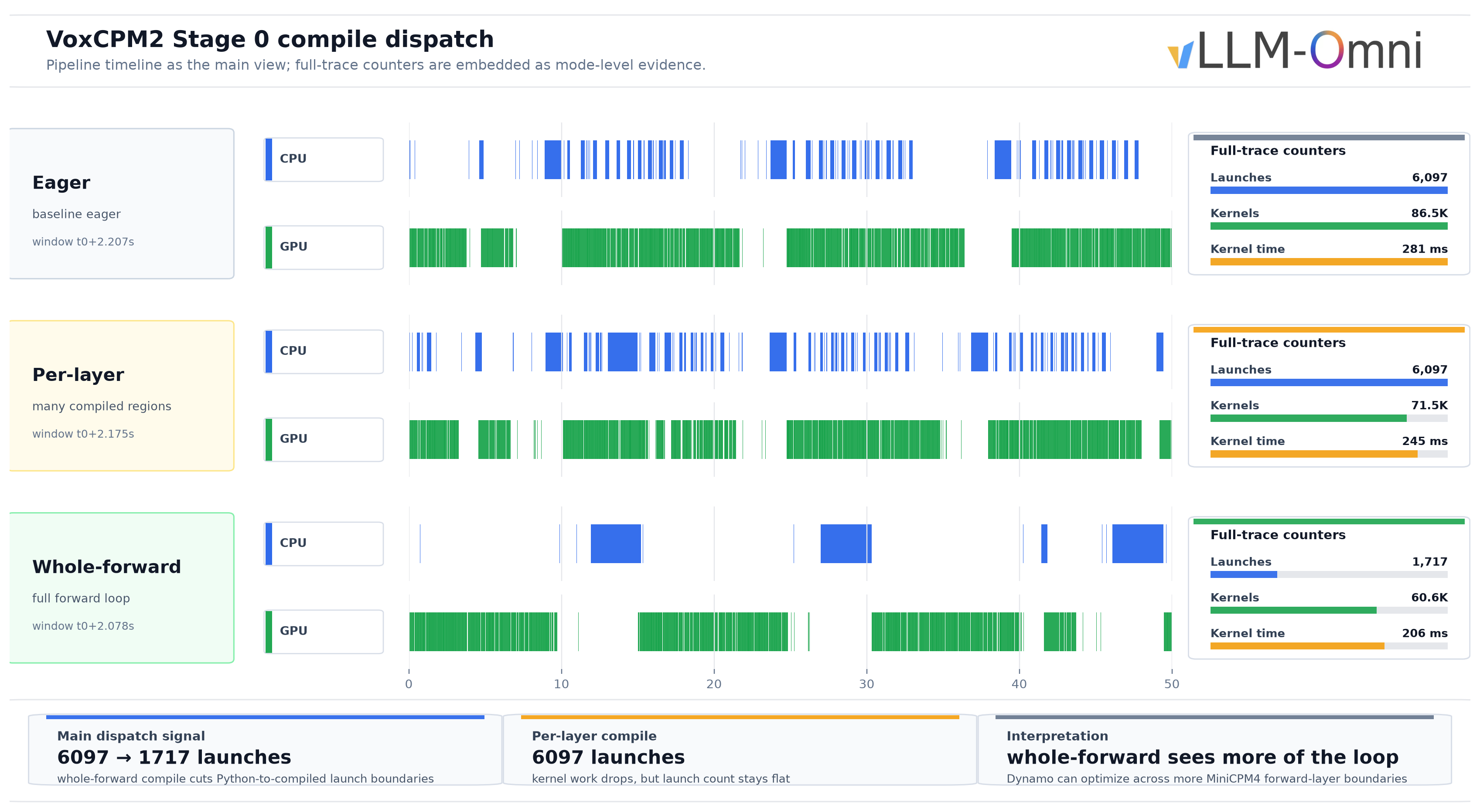
We also tried mode="reduce-overhead", which enables automatic CUDA Graph capture. It conflicted with PagedAttention's stateful KV cache. During graph capture, slot_mapping becomes fixed; replay can then write attention results to the wrong KV cache location, causing incorrect stop logits and early truncation.
fullgraph=True cannot tolerate graph breaks from PagedAttention and custom precision boundaries. fullgraph=False keeps the whole-forward view while allowing those boundaries to fall back to eager execution.
CFM/LocDiT Decode-Tail Batching
After single-request latency improved, the high-concurrency bottleneck moved to CFM/LocDiT. Each request runs a LocDiT attention/GEMM workload during CFM denoising, but the per-request batch is tiny, typically B=2 under CFG. That is far too small to fill the GPU. At high concurrency, requests running LocDiT independently leave the GPU underutilized.
The solution is to batch the CFM/LocDiT decode tail across requests. We collect lm_h, residual outputs, and prefix feature conditions from multiple requests, then run dit_proj, CFM/LocDiT, feat_encoder, and stop_head once as a batch before scattering results back to request state. Combined with VAE decoding every three latent chunks, batched VAE decode, coalesced audio D2H copies, and LocDiT fused-QKV / fused gate-up MLP, H20 × 1 throughput at c=64 improved from 4.19 req/s to 10.83 req/s (+158.8%), and audio throughput improved from 12.16 audio-s/s to 33.07 audio-s/s (+172.0%)8.
There was also a synchronization issue inside the Euler integration loop for CFM. Calling .item() on 0-dim GPU tensors forces GPU-to-CPU synchronization. The original path did this four times per diffusion step. With 10 timesteps and roughly 60 decode steps, one request could trigger around 2,400 synchronizations. Replacing .item() with GPU-side .copy_() broadcasting removes CPU participation from that loop.
VAE decoding had a structural issue as well. The first implementation used an accumulate-and-re-decode pattern: every five steps, it concatenated all previously generated latent patches and decoded the whole prefix again. That makes total work O(N²). Switching to sliding-window decode, with 12 frames of pad context and four new frames per call, reduces the work to O(N). Long-text RTF no longer grows with text length; all lengths stay around RTF 0.132–0.1387.
Higgs Audio V3: Dynamic Batches and Multi-Codebook State
Higgs Audio V3 from Boson AI supports more than 100 languages and zero-shot voice cloning. Architecturally, it has several important features: a Qwen3 backbone with 36 layers and 2560 hidden size, GQA, fused multi-codebook embedding with a large [N × V, D] matrix plus offset lookup, and a MusicGen-style delay pattern [0, 1, 2, ..., 7] with BOC/EOC special tokens.
Its overall Talker → Code2Wav shape is similar to Qwen3-TTS, but the Talker internals are different because of multi-codebook prediction and the delay pattern.
Compared with Qwen3-TTS, Higgs v3 has a different bottleneck. Qwen3-TTS is limited by Python hot paths and streaming chunk boundaries; Higgs v3 is limited by complex multi-codebook decode state management and CUDA Graph compatibility.
Moving Decode State to the GPU
The main Higgs v3 throughput gain came from moving the per-request Python dict state machine into GPU-resident batched tensors9. The state includes _decode_last_codes, _decode_has_codes, delay count, EOC countdown, generation-done flags, and related decode metadata. The benefit comes from reducing Python per-request loops, reducing D2H synchronization, and moving sampling/state update logic onto the batched GPU hot path. In the benchmark reported here, the 35.26 audio-s/s result was measured on a single H20 at c=16 with the eager + local MLP CUDA Graph profile, not the PIECEWISE full-decode graph path.
The hard part is that the vLLM scheduler may reorder, shrink, finish, or remove requests during decode. Row-level state cannot be assumed to equal request-level state. Audio AR state is more complex than text state because delay codebooks, EOC ramp-down, and terminal frames all have semantic meaning. If any state lags by one step, the result is an audio quality problem rather than a clean crash. GPU state, CPU override state, and scheduler tokens must have a single source of truth, or stop semantics become inconsistent.
Adapting CUDA Graph to Dynamic Batch Shapes
CUDA Graph capture for the Higgs v3 Talker decode path exposed another issue. The Talker has an audio feedback mechanism: the embedding of the previous audio token replaces the embedding of the next continuation token. The implementation used a boolean mask to select which requests were currently in decode state. The resulting tensor shape depends on how many requests are in decode state at runtime.
CUDA Graph capture requires fixed stream operations and fixed input/output shapes. A boolean-mask selection whose output shape depends on runtime data violates that requirement.
The workaround is to make the CUDA Graph path use a uniform single-token decode batch. Each span length is 1, so the decode_mask is all True. The selection becomes a no-op and returns the original tensor. The graph sees a stable full-batch shape instead of a data-dependent compacted shape.
Local MLP CUDA Graph vs. PIECEWISE
Local MLP CUDA Graph remains the most important graph optimization for Higgs v3. It covers the main GPU cost in post_attention_layernorm + mlp. vLLM PIECEWISE CUDA Graph looks more complete because it can cover a larger decode step. In practice, Higgs v3's multi-codebook delay pattern makes token layout vary across decode steps. Embedding lookup and pre-attention index operations are data-dependent. PIECEWISE either graph-breaks back to eager in those regions or requires extra metadata synchronization.
In end-to-end tests, PIECEWISE required disabling local MLP graph, and that tradeoff lost more than it gained. Eager plus local MLP graph was faster than PIECEWISE graph.
A Rejected Staging-Overlap Design
One rejected design is still useful to document: one-step audio staging overlap. The idea was to overlap audio-staging D2H copies with the next decode step to reduce GPU idle time. Dry runs passed, but load tests showed that the vLLM scheduler may reorder, shrink, or finish requests during decode. A cursor that points to a row can lose its mapping to a request. This cursor-lag design is structurally unsafe under dynamic batching; it is not a boundary-condition bug. A future overlap design should be request-id keyed and include finish/remove drain hooks.
Fish Speech S2 Pro: When Generic Attention Becomes the Bottleneck
Fish Speech S2 Pro from Fish Audio uses a Dual-AR architecture trained on more than 10 million hours of audio and supports more than 80 languages10. In vLLM-Omni, Fish Speech S2 Pro runs as slow_ar + Fast AR + DAC decoder. slow_ar predicts semantic codebooks along the time axis, Fast AR predicts residual codebooks at each decode step, and the DAC decoder reconstructs waveform audio from 10 codebooks.
Unlike Qwen3-TTS, where Python preprocessing is the main bottleneck, Fish Speech is bottlenecked on the GPU side. At high concurrency, q_len=1 attention dominates. Generic paged/varlen attention carries shape checks and branches for prefill, chunked prefill, decode, and other model shapes. For Fish's pure decode shape, that flexibility is overhead.
Model-Specific Attention Kernel
In profiling, Fish slow_ar at high concurrency spent most of its time in q_len=1 SlowAR attention and in the data handoff between DAC and runtime. Generic attention must support many shapes. Fish decode is much narrower: q_len=1, fp16/bf16, head_dim=128, block size 16, and Fish's GQA layout.
We implemented a Fish-specific Triton kernel for SlowAR decode attention11. It does not handle prefill or other models. If the request does not meet the shape constraints, execution falls back to the original attention path.
The kernel has two paths. Short sequences up to 1024 tokens use standard online softmax in one pass. The grid is (batch_size, num_kv_heads), and each program handles one batch row and one KV head across its Q heads. Block size is hard-coded to 16, matching vLLM's KV cache block size, so block table lookup is a direct tl.load without extra gather logic. Long sequences use a split-partial-combine path: split the sequence into segments, compute partial m/l/acc independently, then merge them using the online softmax recurrence. This keeps reference-audio long-context requests on the fast path.
Dispatch has one subtle detail. The kernel needs sequence length to choose the short or long path, but the exact sequence length lives on GPU. Reading it to CPU would synchronize. Instead, the runner computes a CPU-side seq_lens_cpu_upper_bound from computed tokens plus scheduled tokens. The upper bound is always at least the true sequence length. The short path does not under-read, and the long split path does not under-cover. During CUDA Graph capture, the upper bound is set to max_model_len, so all graph paths remain covered.
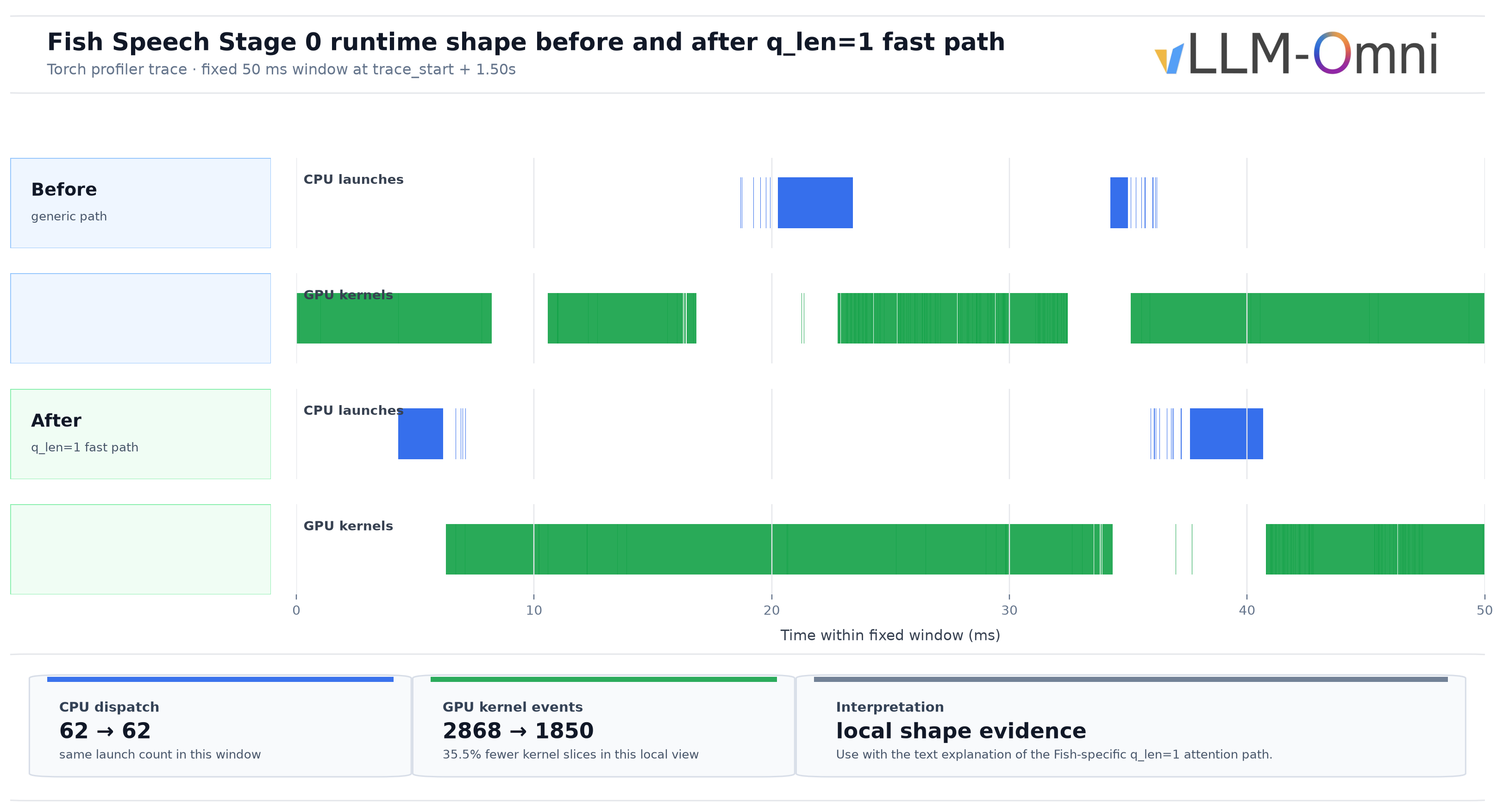
The fast path only applies to Fish SlowAR attention layers. At model load time, we walk model.layers and replace each attention layer's impl.forward with a wrapper that dispatches to the Fish fast path when the constraints match. Prefill requests, non-Fish models, and unsupported decode shapes use the original attention implementation.
Fast AR Buffer Reuse and Compile
Fish Speech Fast AR is a four-layer lightweight transformer that predicts residual codebooks after each slow_ar step. It maintains a per-call KV cache: each residual codebook step only decodes a new token and writes K/V into preallocated _k_cache and _v_cache tensors.
Each Fast AR decode step projects slow_ar hidden state, embeds the current semantic token, runs attention and MLP layer by layer, and samples from logits. Even though the sequence is short, at most 10 tokens, repeated allocation and repeated prefill become visible at c=64.
We allocate _embed_buf, _pos_ids, _k_cache, and _v_cache once and reuse them. _embed_buf has shape (batch_size, num_codebooks + 1, hidden_dim), covering all time steps of one Fast AR decode. _k_cache and _v_cache are preallocated by layer, batch, KV head, sequence position, and head dimension, so forward_one can write and read in place.
We also compile Fast AR with torch.compile. Unlike VoxCPM2 MiniCPM4, Fast AR has only four layers, so compile overhead is small. We use fullgraph=False because attention uses F.scaled_dot_product_attention rather than paged attention, and SDPA may graph-break internally. Dynamo only needs to memoize a few subgraphs. dynamic=True lets the compiled result handle batch-size changes.
DAC and Runtime-Side Optimizations
The DAC and runtime-side changes include several smaller optimizations. Codec payload transfer changed from Python list[int] to tensor payload: a 2D code tensor is serialized directly instead of expanded into Python integers, reducing allocation and GC pressure at high concurrency. fp16 DAC support halves memory and compute. Frame-count-bounded DAC batching caps the number of frames processed in one DAC forward, preventing one long request from blocking others. Async chunk processing overlaps connector transfer and DAC computation: slow_ar and Fast AR produce one 10-codebook codec frame per decode step, the connector batches frames until codec_chunk_frames, and the DAC decoder processes the current chunk while the connector accumulates the next one.
Performance Data
The following numbers come from vLLM-Omni cookbook benchmarks. Metrics:
- RTF: generation time divided by audio duration. Lower than 1 means faster than realtime.
- TTFP: Time To First Audio Packet.
- Tput: audio throughput, or generated audio seconds per wall-clock second.
- E2EL: end-to-end latency.
Qwen3-TTS (c=64, p=512, H20 × 2, voice clone)
| Metric | Before | After | Change |
|---|---|---|---|
| Audio throughput | 26.55 audio-s/s | 42.88 audio-s/s | +61.5% |
| Median E2EL | 9654ms | 5699ms | −41.0% |
| P99 E2EL | 17686ms | 8956ms | −49.4% |
| P99 TTFP | 7558ms | 5563ms | −26.4% |
VoxCPM2 (c=64, H20 × 1, before/after CFM batching)
| Metric | Before | After | Change |
|---|---|---|---|
| Request throughput | 4.19 req/s | 10.83 req/s | +158.8% |
| Audio throughput | 12.16 audio-s/s | 33.07 audio-s/s | +172.0% |
Fish Speech S2 Pro (H20, single GPU, c=64, Triton KV cache + tensor payload)
| Metric | Value |
|---|---|
| Audio throughput | 23.72 audio-s/s |
| Request throughput | 5.95 req/s |
| Mean TTFP | 899.67 ms |
| Mean E2EL | 10.47 s |
Higgs Audio V3 (H20, single GPU, c=16, eager + local MLP graph)
| Metric | Value |
|---|---|
| Request throughput | 5.18 req/s |
| Audio throughput | 35.26 audio-s/s |
| Wall time | 96.5s |
| Speedup vs. baseline | 2.70× |
Acknowledgements
We thank Minghui Jiang, Yueqian Lin, Canlin Guo, Shunyang Li, Taichang Zhou, Yuekai Zhang, Juan Pablo Zuluaga, Nick Cao, Ruirui Yang, Wenjing Chen, Haiyan Wu, Han Gao, Hongsheng Liu, and Roger Wang for their contributions and feedback.
References
If you are interested in TTS inference optimization, join the #sig-omni channel in vLLM Slack, or open an issue in vLLM-Omni GitHub.
Footnotes
-
Qwen3-TTS — QwenLM/Qwen3-TTS ↩
-
VoxCPM2 — OpenBMB/VoxCPM ↩
-
VoxCPM2 whole-model compile + streaming VAE + CFM sync fix — PR #2758 ↩ ↩2
-
VoxCPM2 CFM/LocDiT batching + decode-tail optimizations — PR #3882 ↩
-
Higgs Audio V3 GPU-resident state machine + CUDA Graph — PR #4204 ↩
-
Fish Speech S2 Pro — fishaudio/fish-speech ↩
-
Fish Speech S2 Pro KV cache fast path + DAC optimizations — PR #3773 ↩