

PD Serving of Qwen3.8-2.4T
TL;DR
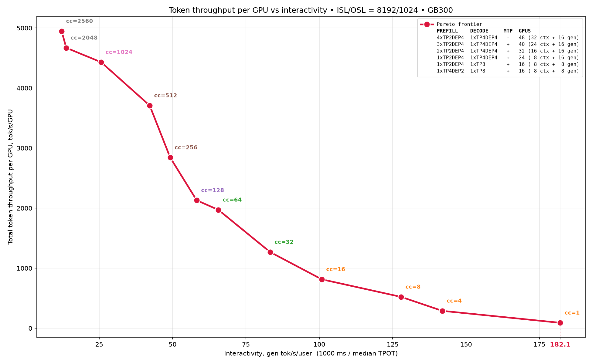
In this blog post we present our latest performance results on PD serving of the Qwen3.8-2.4T model using vLLM on a GB300 NVL72 cluster on 8K/1K workload. In high throughput scenario vLLM achieved 5000 total token throughput per GPU, and 180 generated tokens per user in the low latency scenario — both presented on pareto frontier below. In this blog post we explain in detail how we achieved these results, and give precise srt-slurm recipes to allow anyone to verify and reproduce them using local serving. But what is more important — we describe our decision making process we used to create these recipes. This is even more important than the actual performance results, since it allows you to squeeze performance out of PD serving on vLLM for any model you desire.
Introduction
Recently, we presented our Qwen3.5 PD serving results and showed that vLLM could reach 25K Total TPS/GPU. Straight after that, a new frontier Qwen-family model was released: Qwen3.8-2.4T. In this post, we turn to PD serving for Qwen3.8-2.4T and present the full pareto frontier.
In our previous Qwen3.5 study, we focused primarily on left part of pareto curve, where the goal was to maximize Total TPS/GPU. This time, we go further and build the complete pareto frontier, covering both its left (high throughput) and right (low latency) parts. In other words, besides throughput-oriented configurations, we also identify optimal PD recipes for maximizing interactivity, i.e. Gen TPS per user.
Just as importantly, this blog post is not only about the final numbers. We also break down the tuning process step by step: how we chose what to measure, how we identified bottlenecks, and how we iterated toward better PD configurations. Our aim is to make this workflow understandable and reusable for anyone trying to tune serving performance for any another model.
Maximizing Throughput
The first metric we aim to maximize is total token throughput per GPU. This metric depends on concurrency: more requests a decode engine serves at once, higher throughput we get. What caps concurrency is KV cache capacity, since every active request holds a slice of it. KV cache size is thus the first question to answer for any topology, and it splits in two: how much cache a single request consumes, and how much is left on the GPU once model weight are loaded and vLLM server accocated space for its own work. The rest of this chapter works through both halves and arrives at the maximum concurrency theoretically reachable for Qwen3.8-2.4T on a single GB300.
KV cache estimation for single request
Qwen3.8-2.4T has 92 layers: 69 GDN layers and 23 Full-Attn layers, with an MoE block in every layer (92 × 512 experts). GDN and Full-Attn are BF16, MoE is NVFP4. Weights are classified as follows:
- 91 GiB — non-expert weights of the model (60 GiB for GDN weights and 19 GiB for Full-Attn weights)
- 1242 GiB — expert weights of the model
Since Qwen3.8-2.4T is a hybrid model, its state comes in two parts that are accounted for very differently: Full-Attn state grows with every token, while GDN state is stored per-request.
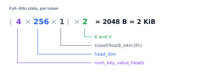
Full-Attn state is stored per token. One token needs 2 KiB per layer:
GDN state is stored per request not per token, this is important. It consists of two parts.
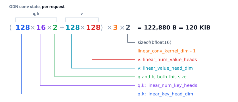
- Conv state — the last kernel-1 inputs of the causal conv, one filter per channel, where the channels are q, k and v concatenated:
- SSM state — recurrent matrix that holds whole context:
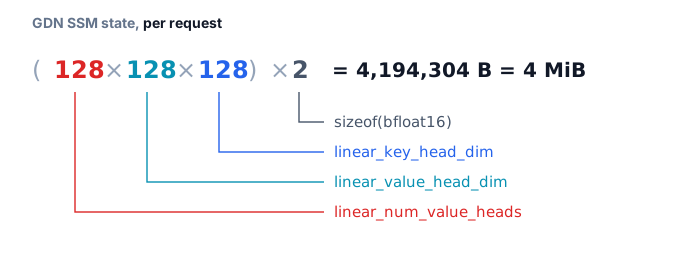
Summing it up, GDN state needs 4 MiB + 120 KiB = 4216 KiB.
vLLM allocates KV cache in blocks, and block has to be large enough to be able to hold either a single GDN state or some number of Full-Attn states. For Qwen3.8-2.4T GDN state dominates Full-Attn state by 4216 KiB / 2 KiB = 2108 times. Block size is then determined by GDN state and aligned to 16 bytes, so align(2108, 16) = 132 * 16 = 2112 tokens fit into one block, making the block 2112 × 2 KiB = 4.125 MiB.
One thing to keep in mind for disaggregated serving: prefill and decode compute their block sizes independently, but KV cache transfer requires both to match. If they do not, set --block-size manually to a value large enough to hold GDN state on both sides, at the cost of some wasted KV cache space.
Now that we calculated size of a single block, we can find out how much KV cache one full request occupies, and from that estimate maximum concurrency we can expect in our measurements. This calculation needs a workload estimation. We fixed ISL=8192 and OSL=1024 — the so-called long-ISL, decode-bound testing scenario.
One request spans ISL, OSL, and a small reserve for chat template used by OpenAI API requests. With 2112 tokens per block, 23 Full-Attn layers and 69 GDN layers, per-request overhead can be calculated this way:
Full-Attn state grows with tokens number, so it needs one block per 2112 tokens in each of the 23 layers. GDN state is fixed per request, so it needs exactly one block in each of the 69 layers. Splitting the total between the two:
KV cache uses GPU memory left over after model loading and all other reservations, so the first step is to determine every memory consumer that allocates memory.
KV cache capacity
GB300 gives us 279 GB to start with. Initially driver overhead takes 2.28 GiB. So, vLLM on start has 276.62 GiB in total. Before the vLLM server starts about 3.13 GiB is already taken by the CUDA context. This is memory we have no control over whatsoever and no way to adjust.
On top of that, by default vLLM reserves 8% of the 276.62 GiB baseline for whatever cannot be predicted in advance — activation memory peak and similar effects. This is what the gpu_memory_utilization setting controls. That already leaves us with ~254 GiB.
Another 2.90 GiB goes into NCCL buffers, allocator and other non-PyTorch related things. So, before weights loading we have 276.62 × 0.92 − 3.13 − 2.90 = 248 GiB.
Peak activations
After weights loading vLLM measures how much memory a model step consumes in eager mode, that is, without CUDA graphs. This is necessary because CUDA graphs themselves are capped at some maximum size, and during inference batch size can exceed that cap — we still have to run the pass somehow, and that is when we need to use eager mode. Such cases are of course worth avoiding as much as possible because of performance degradation, but in practice there is no way to guarantee they never happen in runtime. Eager mode pass is run with max_num_batched_tokens tokens, so that the activation peak is measured in the worst case scenario.
The easiest way for you to estimate memory consumption is to do a few test runs of decode topologies you interested in using aggregated mode. For the topologies covered in this blog post, we got the following peak activations per engine:
| Run | Topology | MTP | max-num-seqs | max-num-batched-tokens | peak activations (GiB) |
|---|---|---|---|---|---|
| 1 | TP8 | + | 20 | 96 | 0.57 |
| 2 | TP8 | + | 32 | 144 | 0.58 |
| 3 | TP8 | + | 80 | 336 | 0.56 |
| 4 | TP8 | + | 272 | 1104 | 1.91 |
| 5 | TP4DP4 | + | 80 | 336 | 1.72 |
| 6 | TP4DP4 | + | 272 | 1104 | 2.24 |
| 7 | TP4DP4 | − | 528 | 544 | 1.83 |
| 8 | TP4DP4 | − | 656 | 672 | 2.15 |
CUDA graphs
After that, vLLM captures CUDA graphs. Memory for graphs must be pre-allocated at static addresses, which means memory that graph needs has to be estimated before the graph will be captured.
By this day vLLM implements this the following way. First we enumerate every graph size available for the server configuration. Only one graph can be replayed at a time, and the larger the graph, the more memory it consumes at peak — so at the very least we must have room for the largest one. The next question is how much extra memory the rest of them need, and here the picture differs from the eager run: once a graph has been captured, replaying it reuses the exact same addresses. Capture the second-largest graph as well and you find that it costs some extra memory
To save warmup time, vLLM then makes the following assumption: that this same
In practice estimate often exceeds the memory graphs actually need by a wide margin. To measure it for yourself, do test runs for decode topologies in aggregated mode with compilation-config: '{"cudagraph_mode": "FULL_DECODE_ONLY"}' with max-cudagraph-capture-size.
For the topologies covered in this blog post, we got the following memory consumption in FULL mode per engine:
| Run | Topology | MTP | # Graphs | Reserved (GiB) | Actually Used (GiB) | Never Used (GiB) | % |
|---|---|---|---|---|---|---|---|
| 1 | TP8 | + | 11 | 0.91 | 0.59 | 0.32 | 54% |
| 2 | TP8 | + | 17 | 1.28 | 0.82 | 0.46 | 56% |
| 3 | TP8 | + | 37 | 1.87 | 1.88 | −0.01 | −1% |
| 4 | TP8 | + | 85 | 7.93 | 6.04 | 1.89 | 31% |
| 5 | TP4DP4 | + | 37 | 8.35 | 6.52 | 1.83 | 28% |
| 6 | TP4DP4 | + | 85 | 7.56 | 9.90 | −2.34 | −24% |
| 7 | TP4DP4 | − | 52 | 8.29 | 7.51 | 0.78 | 10% |
| 8 | TP4DP4 | − | 60 | 8.95 | 8.07 | 0.88 | 11% |
The table also makes it obvious why the gpu_memory_utilization reservation exists in the first place. In some of these runs the memory graphs use more memory that initial estimation, and that extra reservation is exactly what keeps such a case from turning into OOM.
It is important to note that memory space left for KV cache is driven by CUDA graph estimate, not by what graphs actually use in runtime, so KV cache size depends directly on how good that estimate is. In our case it is a good estimate, but if you want to optimize the final percentages, you should probably estimate graphs size manually. Graphs estimation mechanism in vLLM definitely deserves further study and improvement, because with the arrival of over-trillion-parameter frontier models such as Qwen3.8, Kimi-K3 and DSV4 the question becomes pressing.
Maximum concurrency per engine
Now it is time to take all the previous results together and calculate how many requests per engine vLLM can handle for our model. As was said before, GB300 gives us 276.62 GiB. Some of its memory is reserved by gpu_memory_utilization. In our case we used the default value gpu_memory_utilization=0.92. So, initially available memory per engine is 276.62 GiB × 0.92 = 254.5 GiB.
Every column in the table below except the last one is measured: these are the numbers the vLLM server reports at startup. The last column is derived from them — we divide KV cache size by the 759 MiB a single request needs, as computed in KV cache estimation for single request above:
This is a plain division and it deliberately ignores the extra KV slots MTP reserves for speculative tokens, so for MTP rows treat it as an upper bound rather than the concurrency actually reachable.
| Run | Topology | MTP | CUDA ctx (GiB) | non-torch (GiB) | weights (GiB) | peak act (GiB) | graph est (GiB) | KV cache (GiB) | reqs/engine |
|---|---|---|---|---|---|---|---|---|---|
| 1 | TP8 | + | 2.54 | 0.72 | 169.28 | 0.57 | 0.91 | 83.00 | 112.0 |
| 2 | TP8 | + | 2.54 | 0.72 | 169.28 | 0.58 | 1.28 | 82.63 | 111.5 |
| 3 | TP8 | + | 2.54 | 1.19 | 169.28 | 0.56 | 1.87 | 81.60 | 110.1 |
| 4 | TP8 | + | 2.54 | 2.40 | 169.28 | 1.91 | 7.93 | 72.97 | 98.4 |
| 5 | TP4DP4 | + | 3.13 | 1.98 | 108.71 | 1.72 | 8.35 | 133.74 | 180.4 |
| 6 | TP4DP4 | + | 3.13 | 2.22 | 108.71 | 2.24 | 7.56 | 133.77 | 180.5 |
| 7 | TP4DP4 | − | 3.13 | 2.90 | 107.51 | 1.83 | 8.29 | 133.96 | 180.7 |
| 8 | TP4DP4 | − | 3.13 | 3.03 | 107.51 | 2.15 | 8.95 | 132.85 | 179.2 |
From this table we can make several observations. First, in every case we measured, the memory spent on everything that is neither weights nor KV cache comes to ~20 GiB, about 7% of the total memory available. Second, the space given to the model weights varies quite a lot with the topology. Maximizing total token throughput per GPU calls for high concurrency, and concurrency is ultimately limited by the memory available for the KV cache. The only way to free up more of it is to shrink what the model itself requires — which is what makes TP4DP4 the topology to use on decode when chasing top concurrency.
Measure prefill performance
The next important step towards our goal is to measure prefill performance separated from decode. This means running aggregated serving on a prefill-only workload, ISL/OSL=8192/2. This will show us the best topology that we should select for prefill endpoints in disaggregated serving. Such an approach of measuring prefill-only and decode-only workloads separately allows us to select the best topologies and to significantly reduce the amount of work needed for measuring performance of PD serving. In our case we selected the following topologies for prefill:
- TP4DP2+EP
- TP2DP4+EP
- TP4DP4+EP
- TP2DP8+EP
- DP16+EP
- TP1PP6+EP
- TP1PP8+EP
- TP8+EP
- TP16+EP
Here are our measurement results:
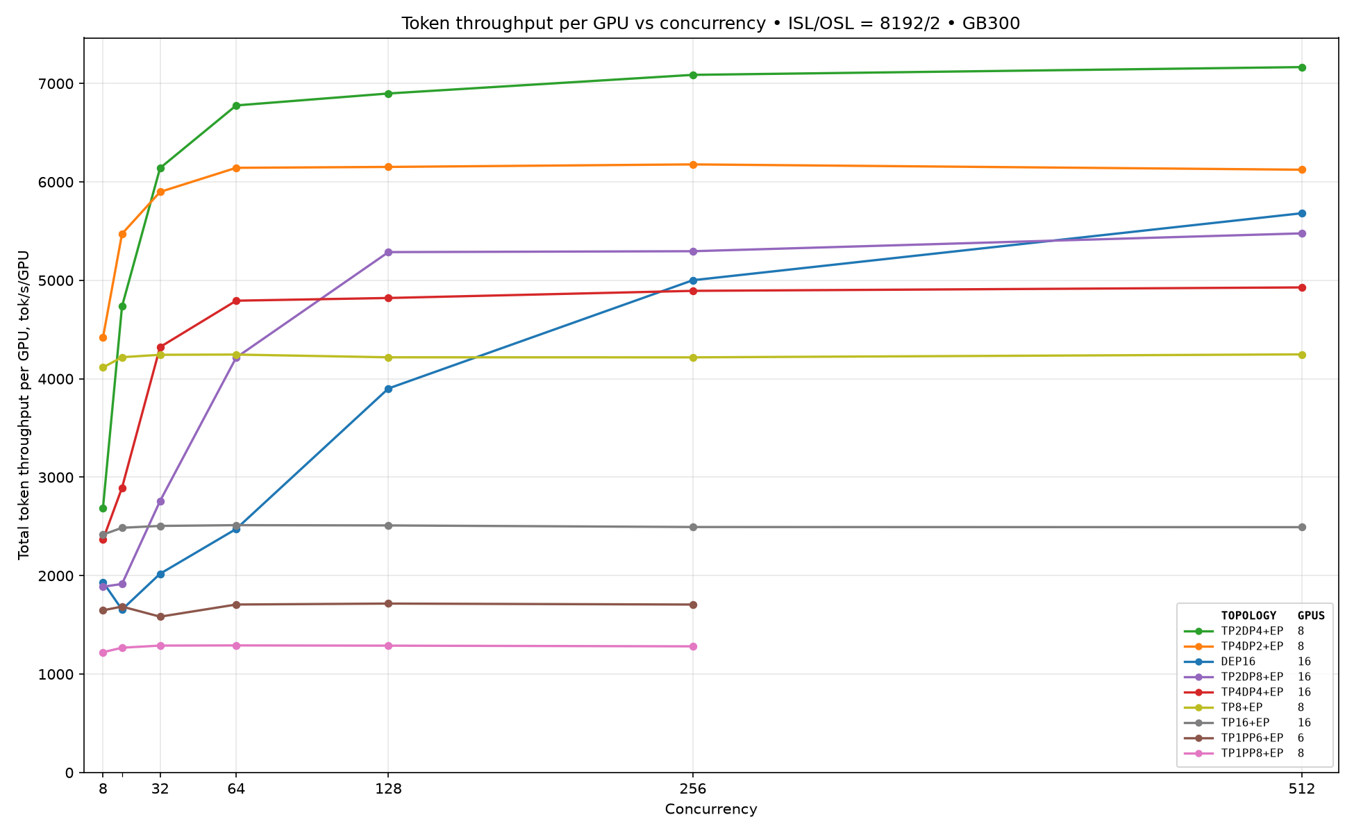
As we can see, for low concurrencies
Measure decode performance
The same thing we do for decode. We run aggregated serving with a decode-only workload, ISL/OSL=1/1000. We selected the following topologies:
- TP2DP4+EP
- TP4DP8+EP
- TEP8
- TEP16
Also, we tried to enable MTP with 3 speculative tokens, as it should help to get better performance results.
Here are our measurement results:
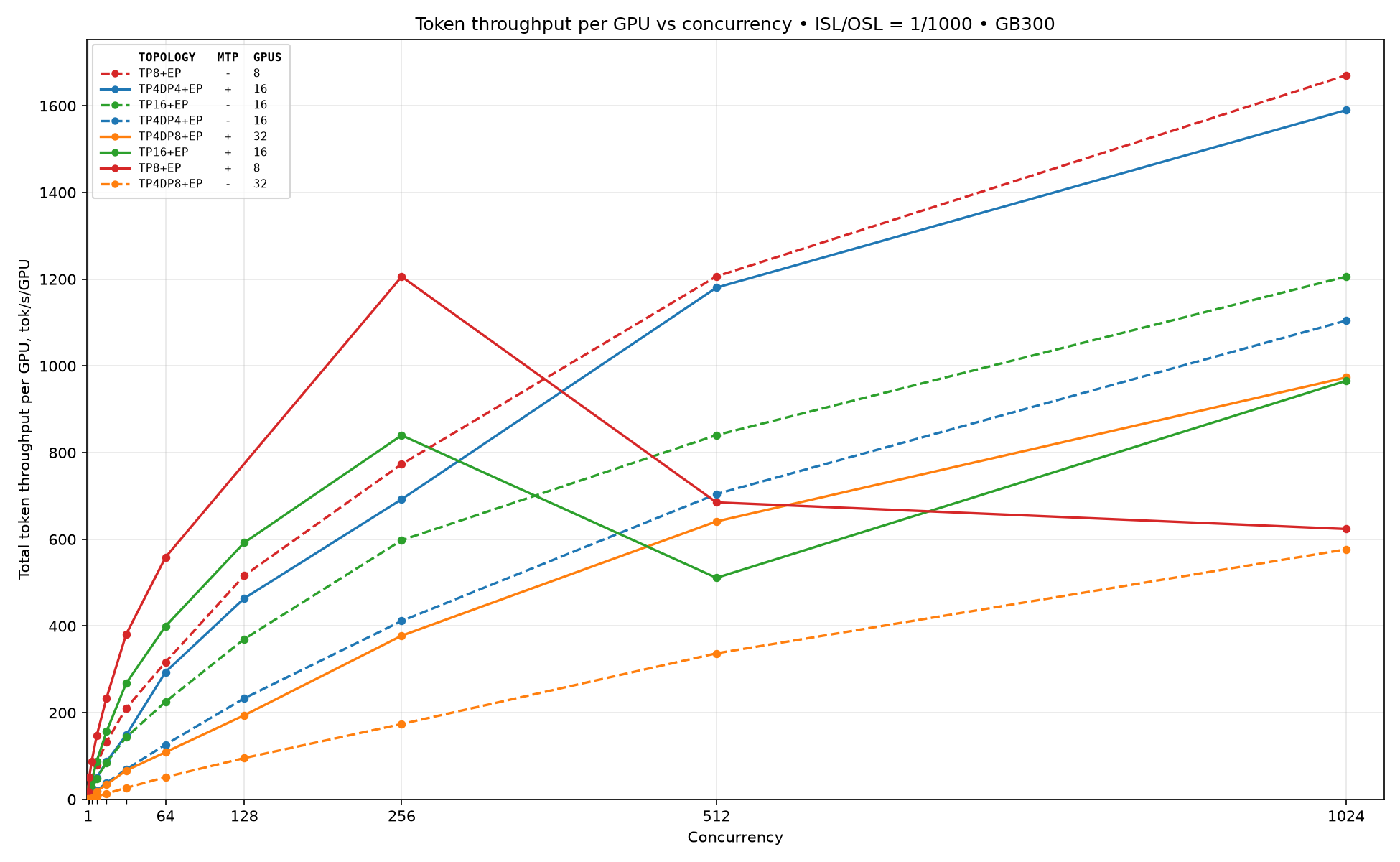
As we can see, firstly MTP drastically improves performance until there is enough available space for KV cache. As well, for concurrencies
Now we have everything required for disaggregated pareto measurements.
Disaggregated Performance Results
Environment Setup
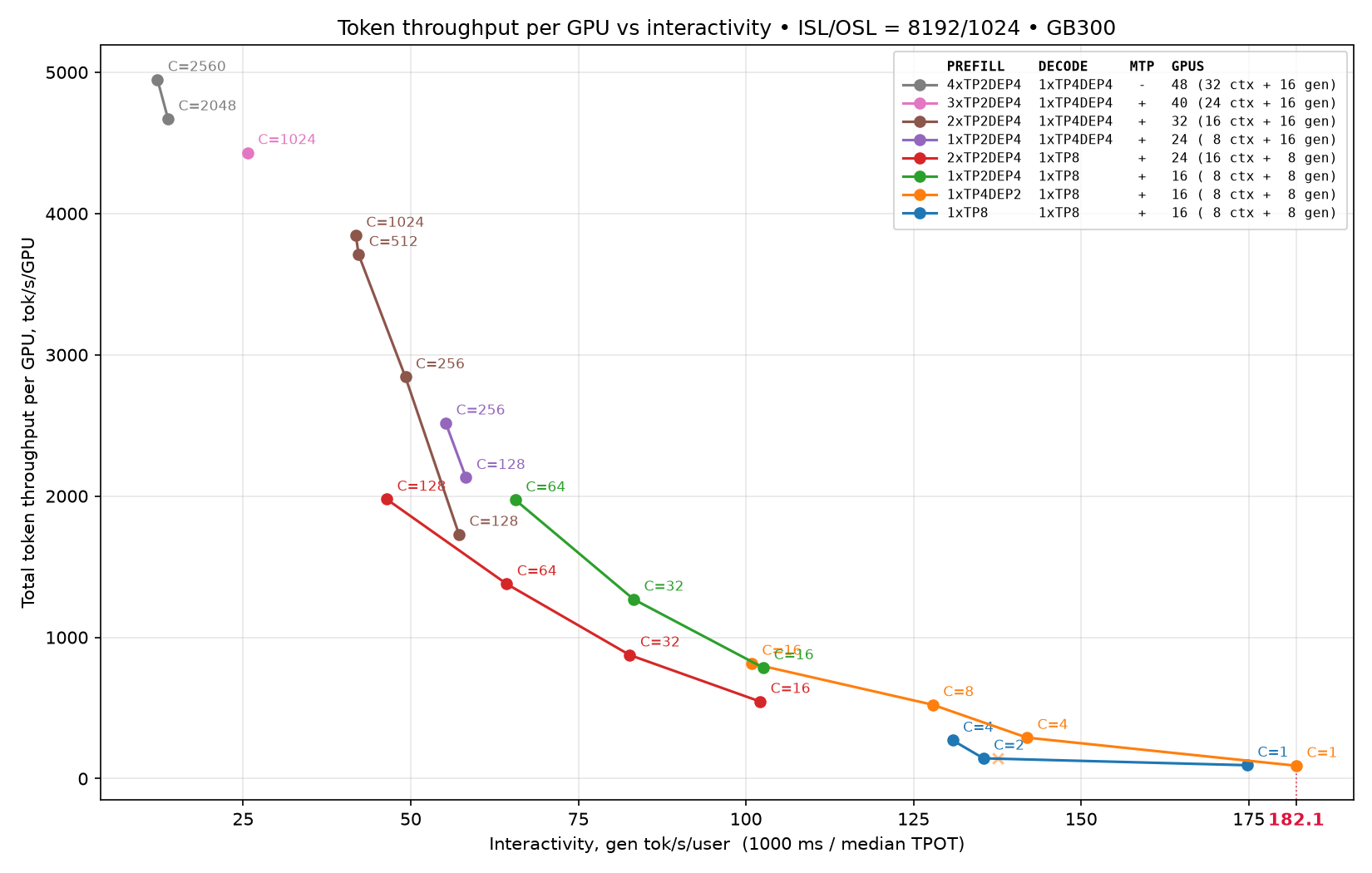
Measurements were conducted on a GB300 cluster connected via NVLink72. We used ISL/OSL = 8192/1024 with concurrency ranging from 1 to 2560. Performance was measured on a fixed decode topology and a constant number of decode endpoints. In this setup, the decode side used one endpoint with 8 or 16 GPUs:
- 1×TEP8
- 1×TP4DP4+EP
On the prefill side, we evaluated configurations ranging from 1 to 4 endpoints, each using from 8 up to 32 GPUs:
- 1×TEP8
- 1×TP4DP2+EP
- {1,2,3,4}×TP2DP4+EP
To reproduce the results, use the Qwen3.8-2.4T NVFP4 model, latest vLLM vllm/vllm-openai:nightly-a9a17 Docker image (vLLM revision v0.26.1rc1.dev1177+ga9a17e709), Dynamo 1.2.0.dev20260526, srt-slurm v1.0.98, and AIPerf utility. All recipes used in this blog post are available in the srt-slurm-recipes repository.
Accuracy Results
The first thing we did was accuracy verification for all the selected configurations of PD serving. Accuracy recipes that you can run yourself using srt-slurm are available in the same repository. We used the standard GSM8K (Grade School Math 8K) benchmark. The final accuracy result is 95% for each PD configuration. Now we can proceed to performance measurements.
Performance Results
Pareto curves for the individual configurations are shown below. Every curve is a single deployment swept over concurrencies, so each point is reachable only by the configuration whose curve it sits on.
Combining all of them gives the final pareto frontier:
Conclusion
In this blog post we showed how such a complex task as building a pareto curve for a frontier Qwen-family model could be decomposed into several smaller independent steps. Finally we reached 5K total token throughput per GPU and interactivity at 180 gen tok/s/user.
Acknowledgements
Artem Perevedentsev (NVIDIA), Vadim Gimpelson (NVIDIA), Xin Li (NVIDIA)
We would also like to thank vLLM community members for contributing and reviewing some optimization efforts mentioned in this blog post.